OOP II: Building Classes¶

Overview¶

In an earlier lecture, we learned some foundations of object-oriented programming.

The objectives of this lecture are

cover OOP in more depth
learn how to build our own objects, specialized to our needs

For example, you already know how to

create lists, strings and other Python objects
use their methods to modify their contents

So imagine now you want to write a program with consumers, who can

hold and spend cash
consume goods
work and earn cash

A natural solution in Python would be to create consumers as objects with

data, such as cash on hand
methods, such as buy or work that affect this data

Python makes it easy to do this, by providing you with class definitions.

Classes are blueprints that help you build objects according to your own specifications.

It takes a little while to get used to the syntax so we’ll provide plenty of examples.

We’ll use the following imports:

import numpy as np
import matplotlib.pyplot as plt
%matplotlib inline

OOP Review¶

OOP is supported in many languages:

JAVA and Ruby are relatively pure OOP.
Python supports both procedural and object-oriented programming.
Fortran and MATLAB are mainly procedural, some OOP recently tacked on.
C is a procedural language, while C++ is C with OOP added on top.

Let’s cover general OOP concepts before we specialize to Python.

Key Concepts¶

As discussed an earlier lecture, in the OOP paradigm, data and functions are bundled together into “objects”.

An example is a Python list, which not only stores data but also knows how to sort itself, etc.

x = [1, 5, 4]
x.sort()
x

[1, 4, 5]

As we now know, sort is a function that is “part of” the list object — and hence called a method.

If we want to make our own types of objects we need to use class definitions.

A class definition is a blueprint for a particular class of objects (e.g., lists, strings or complex numbers).

It describes

What kind of data the class stores
What methods it has for acting on these data

An object or instance is a realization of the class, created from the blueprint

Each instance has its own unique data.
Methods set out in the class definition act on this (and other) data.

In Python, the data and methods of an object are collectively referred to as attributes.

Attributes are accessed via “dotted attribute notation”

object_name.data
object_name.method_name()

In the example

x = [1, 5, 4]
x.sort()
x.__class__

list

x is an object or instance, created from the definition for Python lists, but with its own particular data.
x.sort() and x.__class__ are two attributes of x.
dir(x) can be used to view all the attributes of x.

Why is OOP Useful?¶

OOP is useful for the same reason that abstraction is useful: for recognizing and exploiting the common structure.

For example,

a Markov chain consists of a set of states and a collection of transition probabilities for moving across states
a general equilibrium theory consists of a commodity space, preferences, technologies, and an equilibrium definition
a game consists of a list of players, lists of actions available to each player, player payoffs as functions of all players’ actions, and a timing protocol

These are all abstractions that collect together “objects” of the same “type”.

Recognizing common structure allows us to employ common tools.

In economic theory, this might be a proposition that applies to all games of a certain type.

In Python, this might be a method that’s useful for all Markov chains (e.g., simulate).

When we use OOP, the simulate method is conveniently bundled together with the Markov chain object.

Defining Your Own Classes¶

Let’s build some simple classes to start off.

Example: A Consumer Class¶

First, we’ll build a Consumer class with

a wealth attribute that stores the consumer’s wealth (data)
an earn method, where earn(y) increments the consumer’s wealth by y
a spend method, where spend(x) either decreases wealth by x or returns an error if insufficient funds exist

Admittedly a little contrived, this example of a class helps us internalize some new syntax.

Here’s one implementation

class Consumer:

    def __init__(self, w):
        "Initialize consumer with w dollars of wealth"
        self.wealth = w

    def earn(self, y):
        "The consumer earns y dollars"
        self.wealth += y

    def spend(self, x):
        "The consumer spends x dollars if feasible"
        new_wealth = self.wealth - x
        if new_wealth < 0:
            print("Insufficent funds")
        else:
            self.wealth = new_wealth

There’s some special syntax here so let’s step through carefully

The class keyword indicates that we are building a class.

This class defines instance data wealth and three methods: __init__, earn and spend

wealth is instance data because each consumer we create (each instance of the Consumer class) will have its own separate wealth data.

The ideas behind the earn and spend methods were discussed above.

Both of these act on the instance data wealth.

The __init__ method is a constructor method.

Whenever we create an instance of the class, this method will be called automatically.

Calling __init__ sets up a “namespace” to hold the instance data — more on this soon.

We’ll also discuss the role of self just below.

Usage¶

Here’s an example of usage

c1 = Consumer(10)  # Create instance with initial wealth 10
c1.spend(5)
c1.wealth

c1.earn(15)
c1.spend(100)

Insufficent funds

We can of course create multiple instances each with its own data

c1 = Consumer(10)
c2 = Consumer(12)
c2.spend(4)
c2.wealth

c1.wealth

In fact, each instance stores its data in a separate namespace dictionary

c1.__dict__

{'wealth': 10}

c2.__dict__

{'wealth': 8}

When we access or set attributes we’re actually just modifying the dictionary maintained by the instance.

Self¶

If you look at the Consumer class definition again you’ll see the word self throughout the code.

The rules with self are that

Any instance data should be prepended with self
- e.g., the earn method references self.wealth rather than just wealth
Any method defined within the class should have self as its first argument
- e.g., def earn(self, y) rather than just def earn(y)
Any method referenced within the class should be called as self.method_name

There are no examples of the last rule in the preceding code but we will see some shortly.

Details¶

In this section, we look at some more formal details related to classes and self

You might wish to skip to the next section <oop_solow_growth> on first pass of this lecture.
You can return to these details after you’ve familiarized yourself with more examples.

Methods actually live inside a class object formed when the interpreter reads the class definition

print(Consumer.__dict__)  # Show __dict__ attribute of class object

{'__module__': '__main__', '__init__': <function Consumer.__init__ at 0x7f74b5c31b90>, 'earn': <function Consumer.earn at 0x7f74b5c31c20>, 'spend': <function Consumer.spend at 0x7f74b5c31cb0>, '__dict__': <attribute '__dict__' of 'Consumer' objects>, '__weakref__': <attribute '__weakref__' of 'Consumer' objects>, '__doc__': None}

Note how the three methods __init__, earn and spend are stored in the class object.

Consider the following code

c1 = Consumer(10)
c1.earn(10)
c1.wealth

When you call earn via c1.earn(10) the interpreter passes the instance c1 and the argument 10 to Consumer.earn.

In fact, the following are equivalent

c1.earn(10)
Consumer.earn(c1, 10)

In the function call Consumer.earn(c1, 10) note that c1 is the first argument.

Recall that in the definition of the earn method, self is the first parameter

def earn(self, y):
     "The consumer earns y dollars"
     self.wealth += y

The end result is that self is bound to the instance c1 inside the function call.

That’s why the statement self.wealth += y inside earn ends up modifying c1.wealth.

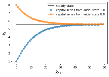
Example: The Solow Growth Model¶

For our next example, let’s write a simple class to implement the Solow growth model.

The Solow growth model is a neoclassical growth model where the amount of capital stock per capita \(k_t\) evolves according to the rule

(2)¶\[k_{t+1} = \frac{s z k_t^{\alpha} + (1 - \delta) k_t}{1 + n}\]

Here

\(s\) is an exogenously given savings rate
\(z\) is a productivity parameter
\(\alpha\) is capital’s share of income
\(n\) is the population growth rate
\(\delta\) is the depreciation rate

The steady state of the model is the \(k\) that solves (2) when \(k_{t+1} = k_t = k\).

Here’s a class that implements this model.

Some points of interest in the code are

An instance maintains a record of its current capital stock in the variable self.k.
The h method implements the right-hand side of (2).
The update method uses h to update capital as per (2).
- Notice how inside update the reference to the local method h is self.h.

The methods steady_state and generate_sequence are fairly self-explanatory

class Solow:
    r"""
    Implements the Solow growth model with the update rule

        k_{t+1} = [(s z k^α_t) + (1 - δ)k_t] /(1 + n)

    """
    def __init__(self, n=0.05,  # population growth rate
                       s=0.25,  # savings rate
                       δ=0.1,   # depreciation rate
                       α=0.3,   # share of labor
                       z=2.0,   # productivity
                       k=1.0):  # current capital stock

        self.n, self.s, self.δ, self.α, self.z = n, s, δ, α, z
        self.k = k

    def h(self):
        "Evaluate the h function"
        # Unpack parameters (get rid of self to simplify notation)
        n, s, δ, α, z = self.n, self.s, self.δ, self.α, self.z
        # Apply the update rule
        return (s * z * self.k**α + (1 - δ) * self.k) / (1 + n)

    def update(self):
        "Update the current state (i.e., the capital stock)."
        self.k =  self.h()

    def steady_state(self):
        "Compute the steady state value of capital."
        # Unpack parameters (get rid of self to simplify notation)
        n, s, δ, α, z = self.n, self.s, self.δ, self.α, self.z
        # Compute and return steady state
        return ((s * z) / (n + δ))**(1 / (1 - α))

    def generate_sequence(self, t):
        "Generate and return a time series of length t"
        path = []
        for i in range(t):
            path.append(self.k)
            self.update()
        return path

Here’s a little program that uses the class to compute time series from two different initial conditions.

The common steady state is also plotted for comparison

s1 = Solow()
s2 = Solow(k=8.0)

T = 60
fig, ax = plt.subplots()

# Plot the common steady state value of capital
ax.plot([s1.steady_state()]*T, 'k-', label='steady state')

# Plot time series for each economy
for s in s1, s2:
    lb = f'capital series from initial state {s.k}'
    ax.plot(s.generate_sequence(T), 'o-', lw=2, alpha=0.6, label=lb)

ax.set_xlabel('$k_{t+1}$', fontsize=14)
ax.set_ylabel('$k_t$', fontsize=14)
ax.legend()
plt.show()

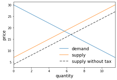
Example: A Market¶

Next, let’s write a class for a simple one good market where agents are price takers.

The market consists of the following objects:

A linear demand curve \(Q = a_d - b_d p\)
A linear supply curve \(Q = a_z + b_z (p - t)\)

Here

\(p\) is price paid by the consumer, \(Q\) is quantity and \(t\) is a per-unit tax.
Other symbols are demand and supply parameters.

The class provides methods to compute various values of interest, including competitive equilibrium price and quantity, tax revenue raised, consumer surplus and producer surplus.

Here’s our implementation.

(It uses a function from SciPy called quad for numerical integration—a topic we will say more about later on.)

from scipy.integrate import quad

class Market:

    def __init__(self, ad, bd, az, bz, tax):
        """
        Set up market parameters.  All parameters are scalars.  See
        https://lectures.quantecon.org/py/python_oop.html for interpretation.

        """
        self.ad, self.bd, self.az, self.bz, self.tax = ad, bd, az, bz, tax
        if ad < az:
            raise ValueError('Insufficient demand.')

    def price(self):
        "Return equilibrium price"
        return  (self.ad - self.az + self.bz * self.tax) / (self.bd + self.bz)

    def quantity(self):
        "Compute equilibrium quantity"
        return  self.ad - self.bd * self.price()

    def consumer_surp(self):
        "Compute consumer surplus"
        # == Compute area under inverse demand function == #
        integrand = lambda x: (self.ad / self.bd) - (1 / self.bd) * x
        area, error = quad(integrand, 0, self.quantity())
        return area - self.price() * self.quantity()

    def producer_surp(self):
        "Compute producer surplus"
        #  == Compute area above inverse supply curve, excluding tax == #
        integrand = lambda x: -(self.az / self.bz) + (1 / self.bz) * x
        area, error = quad(integrand, 0, self.quantity())
        return (self.price() - self.tax) * self.quantity() - area

    def taxrev(self):
        "Compute tax revenue"
        return self.tax * self.quantity()

    def inverse_demand(self, x):
        "Compute inverse demand"
        return self.ad / self.bd - (1 / self.bd)* x

    def inverse_supply(self, x):
        "Compute inverse supply curve"
        return -(self.az / self.bz) + (1 / self.bz) * x + self.tax

    def inverse_supply_no_tax(self, x):
        "Compute inverse supply curve without tax"
        return -(self.az / self.bz) + (1 / self.bz) * x

Here’s a sample of usage

baseline_params = 15, .5, -2, .5, 3
m = Market(*baseline_params)
print("equilibrium price = ", m.price())

equilibrium price =  18.5

print("consumer surplus = ", m.consumer_surp())

consumer surplus =  33.0625

Here’s a short program that uses this class to plot an inverse demand curve together with inverse supply curves with and without taxes

# Baseline ad, bd, az, bz, tax
baseline_params = 15, .5, -2, .5, 3
m = Market(*baseline_params)

q_max = m.quantity() * 2
q_grid = np.linspace(0.0, q_max, 100)
pd = m.inverse_demand(q_grid)
ps = m.inverse_supply(q_grid)
psno = m.inverse_supply_no_tax(q_grid)

fig, ax = plt.subplots()
ax.plot(q_grid, pd, lw=2, alpha=0.6, label='demand')
ax.plot(q_grid, ps, lw=2, alpha=0.6, label='supply')
ax.plot(q_grid, psno, '--k', lw=2, alpha=0.6, label='supply without tax')
ax.set_xlabel('quantity', fontsize=14)
ax.set_xlim(0, q_max)
ax.set_ylabel('price', fontsize=14)
ax.legend(loc='lower right', frameon=False, fontsize=14)
plt.show()

The next program provides a function that

takes an instance of Market as a parameter
computes dead weight loss from the imposition of the tax

def deadw(m):
    "Computes deadweight loss for market m."
    # == Create analogous market with no tax == #
    m_no_tax = Market(m.ad, m.bd, m.az, m.bz, 0)
    # == Compare surplus, return difference == #
    surp1 = m_no_tax.consumer_surp() + m_no_tax.producer_surp()
    surp2 = m.consumer_surp() + m.producer_surp() + m.taxrev()
    return surp1 - surp2

Here’s an example of usage

baseline_params = 15, .5, -2, .5, 3
m = Market(*baseline_params)
deadw(m)  # Show deadweight loss

1.125

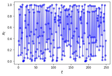
Example: Chaos¶

Let’s look at one more example, related to chaotic dynamics in nonlinear systems.

One simple transition rule that can generate complex dynamics is the logistic map

(3)¶\[x_{t+1} = r x_t(1 - x_t) , \quad x_0 \in [0, 1], \quad r \in [0, 4]\]

Let’s write a class for generating time series from this model.

Here’s one implementation

class Chaos:
  """
  Models the dynamical system with :math:`x_{t+1} = r x_t (1 - x_t)`
  """
  def __init__(self, x0, r):
      """
      Initialize with state x0 and parameter r
      """
      self.x, self.r = x0, r

  def update(self):
      "Apply the map to update state."
      self.x =  self.r * self.x *(1 - self.x)

  def generate_sequence(self, n):
      "Generate and return a sequence of length n."
      path = []
      for i in range(n):
          path.append(self.x)
          self.update()
      return path

Here’s an example of usage

ch = Chaos(0.1, 4.0)     # x0 = 0.1 and r = 0.4
ch.generate_sequence(5)  # First 5 iterates

[0.1, 0.36000000000000004, 0.9216, 0.28901376000000006, 0.8219392261226498]

This piece of code plots a longer trajectory

ch = Chaos(0.1, 4.0)
ts_length = 250

fig, ax = plt.subplots()
ax.set_xlabel('$t$', fontsize=14)
ax.set_ylabel('$x_t$', fontsize=14)
x = ch.generate_sequence(ts_length)
ax.plot(range(ts_length), x, 'bo-', alpha=0.5, lw=2, label='$x_t$')
plt.show()

The next piece of code provides a bifurcation diagram

fig, ax = plt.subplots()
ch = Chaos(0.1, 4)
r = 2.5
while r < 4:
    ch.r = r
    t = ch.generate_sequence(1000)[950:]
    ax.plot([r] * len(t), t, 'b.', ms=0.6)
    r = r + 0.005

ax.set_xlabel('$r$', fontsize=16)
ax.set_ylabel('$x_t$', fontsize=16)
plt.show()

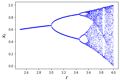
On the horizontal axis is the parameter \(r\) in (3).

The vertical axis is the state space \([0, 1]\).

For each \(r\) we compute a long time series and then plot the tail (the last 50 points).

The tail of the sequence shows us where the trajectory concentrates after settling down to some kind of steady state, if a steady state exists.

Whether it settles down, and the character of the steady state to which it does settle down, depend on the value of \(r\).

For \(r\) between about 2.5 and 3, the time series settles into a single fixed point plotted on the vertical axis.

For \(r\) between about 3 and 3.45, the time series settles down to oscillating between the two values plotted on the vertical axis.

For \(r\) a little bit higher than 3.45, the time series settles down to oscillating among the four values plotted on the vertical axis.

Notice that there is no value of \(r\) that leads to a steady state oscillating among three values.

Special Methods¶

Python provides special methods with which some neat tricks can be performed.

For example, recall that lists and tuples have a notion of length and that this length can be queried via the len function

x = (10, 20)
len(x)

If you want to provide a return value for the len function when applied to your user-defined object, use the __len__ special method

class Foo:

    def __len__(self):
        return 42

Now we get

f = Foo()
len(f)

A special method we will use regularly is the __call__ method.

This method can be used to make your instances callable, just like functions

class Foo:

    def __call__(self, x):
        return x + 42

After running we get

f = Foo()
f(8)  # Exactly equivalent to f.__call__(8)

Exercise 1 provides a more useful example.

Exercises¶

Exercise 1¶

The empirical cumulative distribution function (ecdf) corresponding to a sample \(\{X_i\}_{i=1}^n\) is defined as

(4)¶\[F_n(x) := \frac{1}{n} \sum_{i=1}^n \mathbf{1}\{X_i \leq x\} \qquad (x \in \mathbb{R})\]

Here \(\mathbf{1}\{X_i \leq x\}\) is an indicator function (one if \(X_i \leq x\) and zero otherwise) and hence \(F_n(x)\) is the fraction of the sample that falls below \(x\).

The Glivenko–Cantelli Theorem states that, provided that the sample is IID, the ecdf \(F_n\) converges to the true distribution function \(F\).

Implement \(F_n\) as a class called ECDF, where

A given sample \(\{X_i\}_{i=1}^n\) are the instance data, stored as self.observations.
The class implements a __call__ method that returns \(F_n(x)\) for any \(x\).

Your code should work as follows (modulo randomness)

from random import uniform

samples = [uniform(0, 1) for i in range(10)]
F = ECDF(samples)
F(0.5)  # Evaluate ecdf at x = 0.5

F.observations = [uniform(0, 1) for i in range(1000)]
F(0.5)

Aim for clarity, not efficiency.

Exercise 2¶

In an earlier exercise, you wrote a function for evaluating polynomials.

This exercise is an extension, where the task is to build a simple class called Polynomial for representing and manipulating polynomial functions such as

(5)¶\[p(x) = a_0 + a_1 x + a_2 x^2 + \cdots a_N x^N = \sum_{n=0}^N a_n x^n \qquad (x \in \mathbb{R})\]

The instance data for the class Polynomial will be the coefficients (in the case of (5), the numbers \(a_0, \ldots, a_N\)).

Provide methods that

Evaluate the polynomial (5), returning \(p(x)\) for any \(x\).
Differentiate the polynomial, replacing the original coefficients with those of its derivative \(p'\).

Avoid using any import statements.

Solutions¶

Exercise 1¶

class ECDF:

    def __init__(self, observations):
        self.observations = observations

    def __call__(self, x):
        counter = 0.0
        for obs in self.observations:
            if obs <= x:
                counter += 1
        return counter / len(self.observations)

# == test == #

from random import uniform

samples = [uniform(0, 1) for i in range(10)]
F = ECDF(samples)

print(F(0.5))  # Evaluate ecdf at x = 0.5

F.observations = [uniform(0, 1) for i in range(1000)]

print(F(0.5))

0.4
0.487

Exercise 2¶

class Polynomial:

    def __init__(self, coefficients):
        """
        Creates an instance of the Polynomial class representing

            p(x) = a_0 x^0 + ... + a_N x^N,

        where a_i = coefficients[i].
        """
        self.coefficients = coefficients

    def __call__(self, x):
        "Evaluate the polynomial at x."
        y = 0
        for i, a in enumerate(self.coefficients):
            y += a * x**i
        return y

    def differentiate(self):
        "Reset self.coefficients to those of p' instead of p."
        new_coefficients = []
        for i, a in enumerate(self.coefficients):
            new_coefficients.append(i * a)
        # Remove the first element, which is zero
        del new_coefficients[0]
        # And reset coefficients data to new values
        self.coefficients = new_coefficients
        return new_coefficients

Programming for Quantitative Economics

OOP II: Building Classes¶

Overview¶

OOP Review¶

Key Concepts¶

Why is OOP Useful?¶

Defining Your Own Classes¶

Example: A Consumer Class¶

Usage¶

Self¶

Details¶

Example: The Solow Growth Model¶

Example: A Market¶

Example: Chaos¶

Special Methods¶

Exercises¶

Exercise 1¶

Exercise 2¶

Solutions¶

Exercise 1¶

Exercise 2¶