.ipynb .md .pdf

repository suggest edit

Binder

Contents

Pandas

In addition to what’s in Anaconda, this lecture will need the following libraries:

!pip install --upgrade pandas-datareader

Overview

Pandas is a package of fast, efficient data analysis tools for Python.

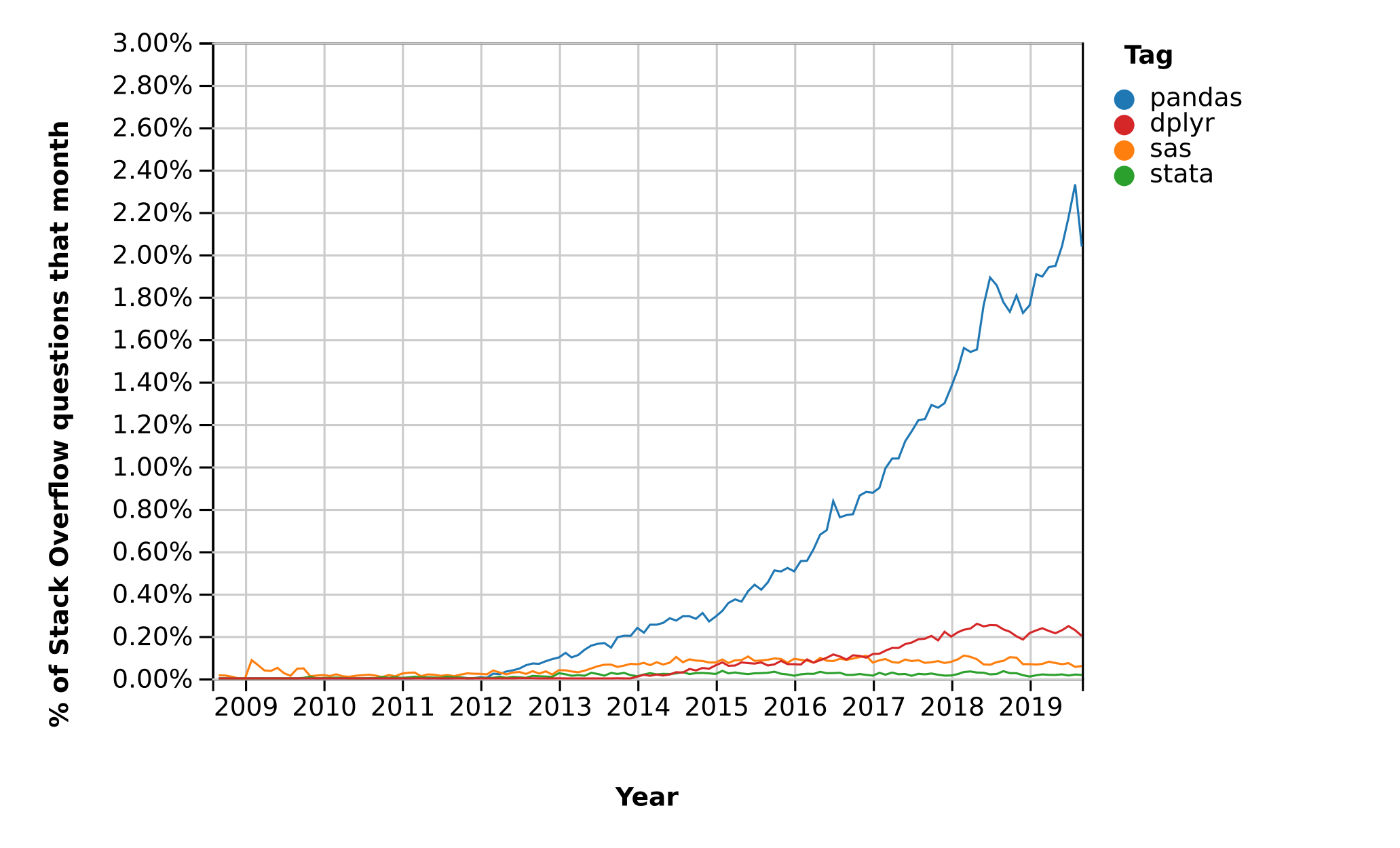
Its popularity has surged in recent years, coincident with the rise of fields such as data science and machine learning.

Here’s a popularity comparison over time against STATA, SAS, and dplyr courtesy of Stack Overflow Trends

Just as NumPy provides the basic array data type plus core array operations, pandas

1. defines fundamental structures for working with data and

2. endows them with methods that facilitate operations such as

• reading in data

• adjusting indices

• working with dates and time series

• sorting, grouping, re-ordering and general data munging2

• dealing with missing values, etc., etc.

More sophisticated statistical functionality is left to other packages, such as statsmodels and scikit-learn, which are built on top of pandas.

This lecture will provide a basic introduction to pandas.

Throughout the lecture, we will assume that the following imports have taken place

import pandas as pd
import numpy as np
import matplotlib.pyplot as plt
%matplotlib inline
import requests

Series

Two important data types defined by pandas are Series and DataFrame.

You can think of a Series as a “column” of data, such as a collection of observations on a single variable.

A DataFrame is an object for storing related columns of data.

Let’s start with Series

s = pd.Series(np.random.randn(4), name='daily returns')
s

0   -1.429498
1   -0.239781
2    0.045972
3   -1.261449
Name: daily returns, dtype: float64

Here you can imagine the indices 0, 1, 2, 3 as indexing four listed companies, and the values being daily returns on their shares.

Pandas Series are built on top of NumPy arrays and support many similar operations

s * 100

0   -142.949832
1    -23.978093
2      4.597185
3   -126.144901
Name: daily returns, dtype: float64

np.abs(s)

0    1.429498
1    0.239781
2    0.045972
3    1.261449
Name: daily returns, dtype: float64

But Series provide more than NumPy arrays.

Not only do they have some additional (statistically oriented) methods

s.describe()

count    4.000000
mean    -0.721189
std      0.733456
min     -1.429498
25%     -1.303461
50%     -0.750615
75%     -0.168343
max      0.045972
Name: daily returns, dtype: float64

But their indices are more flexible

s.index = ['AMZN', 'AAPL', 'MSFT', 'GOOG']
s

AMZN   -1.429498
AAPL   -0.239781
MSFT    0.045972
GOOG   -1.261449
Name: daily returns, dtype: float64

Viewed in this way, Series are like fast, efficient Python dictionaries (with the restriction that the items in the dictionary all have the same type—in this case, floats).

In fact, you can use much of the same syntax as Python dictionaries

s['AMZN']

-1.4294983173008147

s['AMZN'] = 0
s

AMZN    0.000000
AAPL   -0.239781
MSFT    0.045972
GOOG   -1.261449
Name: daily returns, dtype: float64

'AAPL' in s

True

DataFrames

While a Series is a single column of data, a DataFrame is several columns, one for each variable.

In essence, a DataFrame in pandas is analogous to a (highly optimized) Excel spreadsheet.

Thus, it is a powerful tool for representing and analyzing data that are naturally organized into rows and columns, often with descriptive indexes for individual rows and individual columns.

Let’s look at an example that reads data from the CSV file pandas/data/test_pwt.csv that can be downloaded here.

Here’s the content of test_pwt.csv

"country","country isocode","year","POP","XRAT","tcgdp","cc","cg"
"Argentina","ARG","2000","37335.653","0.9995","295072.21869","75.716805379","5.5788042896"
"Australia","AUS","2000","19053.186","1.72483","541804.6521","67.759025993","6.7200975332"
"India","IND","2000","1006300.297","44.9416","1728144.3748","64.575551328","14.072205773"
"Israel","ISR","2000","6114.57","4.07733","129253.89423","64.436450847","10.266688415"
"Malawi","MWI","2000","11801.505","59.543808333","5026.2217836","74.707624181","11.658954494"
"South Africa","ZAF","2000","45064.098","6.93983","227242.36949","72.718710427","5.7265463933"
"United States","USA","2000","282171.957","1","9898700","72.347054303","6.0324539789"
"Uruguay","URY","2000","3219.793","12.099591667","25255.961693","78.978740282","5.108067988"

Supposing you have this data saved as test_pwt.csv in the present working directory (type %pwd in Jupyter to see what this is), it can be read in as follows:

df = pd.read_csv('https://raw.githubusercontent.com/QuantEcon/lecture-source-py/master/source/_static/lecture_specific/pandas/data/test_pwt.csv')
type(df)

pandas.core.frame.DataFrame

df

	country	country isocode	year	POP	XRAT	tcgdp	cc	cg
0	Argentina	ARG	2000	37335.653	0.999500	2.950722e+05	75.716805	5.578804
1	Australia	AUS	2000	19053.186	1.724830	5.418047e+05	67.759026	6.720098
2	India	IND	2000	1006300.297	44.941600	1.728144e+06	64.575551	14.072206
3	Israel	ISR	2000	6114.570	4.077330	1.292539e+05	64.436451	10.266688
4	Malawi	MWI	2000	11801.505	59.543808	5.026222e+03	74.707624	11.658954
5	South Africa	ZAF	2000	45064.098	6.939830	2.272424e+05	72.718710	5.726546
6	United States	USA	2000	282171.957	1.000000	9.898700e+06	72.347054	6.032454
7	Uruguay	URY	2000	3219.793	12.099592	2.525596e+04	78.978740	5.108068

We can select particular rows using standard Python array slicing notation

df[2:5]

	country	country isocode	year	POP	XRAT	tcgdp	cc	cg
2	India	IND	2000	1006300.297	44.941600	1.728144e+06	64.575551	14.072206
3	Israel	ISR	2000	6114.570	4.077330	1.292539e+05	64.436451	10.266688
4	Malawi	MWI	2000	11801.505	59.543808	5.026222e+03	74.707624	11.658954

To select columns, we can pass a list containing the names of the desired columns represented as strings

df[['country', 'tcgdp']]

	country	tcgdp
0	Argentina	2.950722e+05
1	Australia	5.418047e+05
2	India	1.728144e+06
3	Israel	1.292539e+05
4	Malawi	5.026222e+03
5	South Africa	2.272424e+05
6	United States	9.898700e+06
7	Uruguay	2.525596e+04

To select both rows and columns using integers, the iloc attribute should be used with the format .iloc[rows, columns]

df.iloc[2:5, 0:4]

	country	country isocode	year	POP
2	India	IND	2000	1006300.297
3	Israel	ISR	2000	6114.570
4	Malawi	MWI	2000	11801.505

To select rows and columns using a mixture of integers and labels, the loc attribute can be used in a similar way

df.loc[df.index[2:5], ['country', 'tcgdp']]

	country	tcgdp
2	India	1.728144e+06
3	Israel	1.292539e+05
4	Malawi	5.026222e+03

Let’s imagine that we’re only interested in population (POP) and total GDP (tcgdp).

One way to strip the data frame df down to only these variables is to overwrite the dataframe using the selection method described above

df = df[['country', 'POP', 'tcgdp']]
df

	country	POP	tcgdp
0	Argentina	37335.653	2.950722e+05
1	Australia	19053.186	5.418047e+05
2	India	1006300.297	1.728144e+06
3	Israel	6114.570	1.292539e+05
4	Malawi	11801.505	5.026222e+03
5	South Africa	45064.098	2.272424e+05
6	United States	282171.957	9.898700e+06
7	Uruguay	3219.793	2.525596e+04

Here the index 0, 1,..., 7 is redundant because we can use the country names as an index.

To do this, we set the index to be the country variable in the dataframe

df = df.set_index('country')
df

	POP	tcgdp
country
Argentina	37335.653	2.950722e+05
Australia	19053.186	5.418047e+05
India	1006300.297	1.728144e+06
Israel	6114.570	1.292539e+05
Malawi	11801.505	5.026222e+03
South Africa	45064.098	2.272424e+05
United States	282171.957	9.898700e+06
Uruguay	3219.793	2.525596e+04

Let’s give the columns slightly better names

df.columns = 'population', 'total GDP'
df

	population	total GDP
country
Argentina	37335.653	2.950722e+05
Australia	19053.186	5.418047e+05
India	1006300.297	1.728144e+06
Israel	6114.570	1.292539e+05
Malawi	11801.505	5.026222e+03
South Africa	45064.098	2.272424e+05
United States	282171.957	9.898700e+06
Uruguay	3219.793	2.525596e+04

Population is in thousands, let’s revert to single units

df['population'] = df['population'] * 1e3
df

	population	total GDP
country
Argentina	3.733565e+07	2.950722e+05
Australia	1.905319e+07	5.418047e+05
India	1.006300e+09	1.728144e+06
Israel	6.114570e+06	1.292539e+05
Malawi	1.180150e+07	5.026222e+03
South Africa	4.506410e+07	2.272424e+05
United States	2.821720e+08	9.898700e+06
Uruguay	3.219793e+06	2.525596e+04

Next, we’re going to add a column showing real GDP per capita, multiplying by 1,000,000 as we go because total GDP is in millions

df['GDP percap'] = df['total GDP'] * 1e6 / df['population']
df

	population	total GDP	GDP percap
country
Argentina	3.733565e+07	2.950722e+05	7903.229085
Australia	1.905319e+07	5.418047e+05	28436.433261
India	1.006300e+09	1.728144e+06	1717.324719
Israel	6.114570e+06	1.292539e+05	21138.672749
Malawi	1.180150e+07	5.026222e+03	425.896679
South Africa	4.506410e+07	2.272424e+05	5042.647686
United States	2.821720e+08	9.898700e+06	35080.381854
Uruguay	3.219793e+06	2.525596e+04	7843.970620

One of the nice things about pandas DataFrame and Series objects is that they have methods for plotting and visualization that work through Matplotlib.

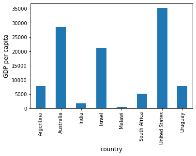
For example, we can easily generate a bar plot of GDP per capita

ax = df['GDP percap'].plot(kind='bar')
ax.set_xlabel('country', fontsize=12)
ax.set_ylabel('GDP per capita', fontsize=12)
plt.show()

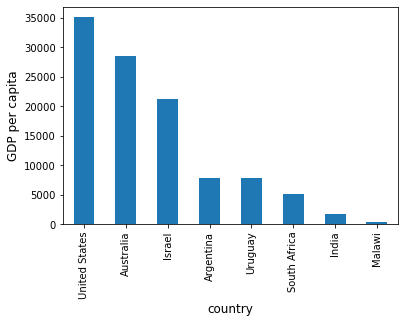
At the moment the data frame is ordered alphabetically on the countries—let’s change it to GDP per capita

df = df.sort_values(by='GDP percap', ascending=False)
df

	population	total GDP	GDP percap
country
United States	2.821720e+08	9.898700e+06	35080.381854
Australia	1.905319e+07	5.418047e+05	28436.433261
Israel	6.114570e+06	1.292539e+05	21138.672749
Argentina	3.733565e+07	2.950722e+05	7903.229085
Uruguay	3.219793e+06	2.525596e+04	7843.970620
South Africa	4.506410e+07	2.272424e+05	5042.647686
India	1.006300e+09	1.728144e+06	1717.324719
Malawi	1.180150e+07	5.026222e+03	425.896679

Plotting as before now yields

ax = df['GDP percap'].plot(kind='bar')
ax.set_xlabel('country', fontsize=12)
ax.set_ylabel('GDP per capita', fontsize=12)
plt.show()

On-Line Data Sources

Python makes it straightforward to query online databases programmatically.

An important database for economists is FRED — a vast collection of time series data maintained by the St. Louis Fed.

For example, suppose that we are interested in the unemployment rate.

Via FRED, the entire series for the US civilian unemployment rate can be downloaded directly by entering this URL into your browser (note that this requires an internet connection)

https://research.stlouisfed.org/fred2/series/UNRATE/downloaddata/UNRATE.csv

(Equivalently, click here: https://research.stlouisfed.org/fred2/series/UNRATE/downloaddata/UNRATE.csv)

This request returns a CSV file, which will be handled by your default application for this class of files.

Alternatively, we can access the CSV file from within a Python program.

This can be done with a variety of methods.

We start with a relatively low-level method and then return to pandas.

Accessing Data with requests

One option is to use requests, a standard Python library for requesting data over the Internet.

To begin, try the following code on your computer

r = requests.get('http://research.stlouisfed.org/fred2/series/UNRATE/downloaddata/UNRATE.csv')

If there’s no error message, then the call has succeeded.

If you do get an error, then there are two likely causes

1. You are not connected to the Internet — hopefully, this isn’t the case.

2. Your machine is accessing the Internet through a proxy server, and Python isn’t aware of this.

In the second case, you can either

• switch to another machine

• solve your proxy problem by reading the documentation

Assuming that all is working, you can now proceed to use the source object returned by the call requests.get('http://research.stlouisfed.org/fred2/series/UNRATE/downloaddata/UNRATE.csv')

url = 'http://research.stlouisfed.org/fred2/series/UNRATE/downloaddata/UNRATE.csv'
source = requests.get(url).content.decode().split("\n")
source[0]

'DATE,VALUE\r'

source[1]

'1948-01-01,3.4\r'

source[2]

'1948-02-01,3.8\r'

We could now write some additional code to parse this text and store it as an array.

But this is unnecessary — pandas’ read_csv function can handle the task for us.

We use parse_dates=True so that pandas recognizes our dates column, allowing for simple date filtering

data = pd.read_csv(url, index_col=0, parse_dates=True)

The data has been read into a pandas DataFrame called data that we can now manipulate in the usual way

type(data)

pandas.core.frame.DataFrame

data.head()  # A useful method to get a quick look at a data frame

	VALUE
DATE
1948-01-01	3.4
1948-02-01	3.8
1948-03-01	4.0
1948-04-01	3.9
1948-05-01	3.5

pd.set_option('precision', 1)
data.describe()  # Your output might differ slightly

	VALUE
count	873.0
mean	5.8
std	1.7
min	2.5
25%	4.5
50%	5.6
75%	6.8
max	14.7

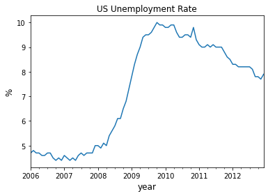
We can also plot the unemployment rate from 2006 to 2012 as follows

ax = data['2006':'2012'].plot(title='US Unemployment Rate', legend=False)
ax.set_xlabel('year', fontsize=12)
ax.set_ylabel('%', fontsize=12)
plt.show()

Note that pandas offers many other file type alternatives.

Pandas has a wide variety of top-level methods that we can use to read, excel, json, parquet or plug straight into a database server.

Using pandas_datareader to Access Data

The maker of pandas has also authored a library called pandas_datareader that gives programmatic access to many data sources straight from the Jupyter notebook.

While some sources require an access key, many of the most important (e.g., FRED, OECD, EUROSTAT and the World Bank) are free to use.

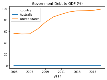
For now let’s work through one example of downloading and plotting data — this time from the World Bank.

The World Bank collects and organizes data on a huge range of indicators.

For example, here’s some data on government debt as a ratio to GDP.

The next code example fetches the data for you and plots time series for the US and Australia

from pandas_datareader import wb

govt_debt = wb.download(indicator='GC.DOD.TOTL.GD.ZS', country=['US', 'AU'], start=2005, end=2016).stack().unstack(0)
ind = govt_debt.index.droplevel(-1)
govt_debt.index = ind
ax = govt_debt.plot(lw=2)
ax.set_xlabel('year', fontsize=12)
plt.title("Government Debt to GDP (%)")
plt.show()

The documentation provides more details on how to access various data sources.

Exercises

Exercise 1

With these imports:

import datetime as dt 
from pandas_datareader import data

Write a program to calculate the percentage price change over 2019 for the following shares:

ticker_list = {'INTC': 'Intel',
               'MSFT': 'Microsoft',
               'IBM': 'IBM',
               'BHP': 'BHP',
               'TM': 'Toyota',
               'AAPL': 'Apple',
               'AMZN': 'Amazon',
               'BA': 'Boeing',
               'QCOM': 'Qualcomm',
               'KO': 'Coca-Cola',
               'GOOG': 'Google',
               'SNE': 'Sony',
               'PTR': 'PetroChina'}

Here’s the first part of the program

def read_data(ticker_list,
          start=dt.datetime(2019, 1, 2),
          end=dt.datetime(2019, 12, 31)): 
    """
    This function reads in closing price data from Yahoo 
    for each tick in the ticker_list.
    """
    ticker = pd.DataFrame()

    for tick in ticker_list:
        prices = data.DataReader(tick, 'yahoo', start, end)
        closing_prices = prices['Close']
        ticker[tick] = closing_prices

    return ticker

ticker = read_data(ticker_list)

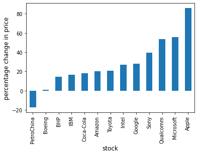
Complete the program to plot the result as a bar graph like this one:

Exercise 2

Using the method read_data introduced in Exercise 1, write a program to obtain year-on-year percentage change for the following indices:

indices_list = {'^GSPC': 'S&P 500',
               '^IXIC': 'NASDAQ',
               '^DJI': 'Dow Jones',
               '^N225': 'Nikkei'}

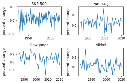
Complete the program to show summary statistics and plot the result as a time series graph like this one:

Solutions

Exercise 1

There are a few ways to approach this problem using Pandas to calculate the percentage change.

First, you can extract the data and perform the calculation such as:

p1 = ticker.iloc[0]    #Get the first set of prices as a Series
p2 = ticker.iloc[-1]   #Get the last set of prices as a Series
price_change = (p2 - p1) / p1 * 100
price_change

INTC    27.1
MSFT    56.0
IBM     16.3
BHP     14.3
TM      20.9
AAPL    85.9
AMZN    20.1
BA       0.6
QCOM    53.7
KO      17.9
GOOG    27.8
SNE     39.6
PTR    -17.4
dtype: float64

Alternatively you can use an inbuilt method pct_change and configure it to perform the correct calculation using periods argument.

change = ticker.pct_change(periods=len(ticker)-1, axis='rows')*100
price_change = change.iloc[-1]
price_change

INTC    27.1
MSFT    56.0
IBM     16.3
BHP     14.3
TM      20.9
AAPL    85.9
AMZN    20.1
BA       0.6
QCOM    53.7
KO      17.9
GOOG    27.8
SNE     39.6
PTR    -17.4
Name: 2019-12-31 00:00:00, dtype: float64

Then to plot the chart

price_change.sort_values(inplace=True)
price_change = price_change.rename(index=ticker_list)
fig, ax = plt.subplots()
ax.set_xlabel('stock', fontsize=12)
ax.set_ylabel('percentage change in price', fontsize=12)
price_change.plot(kind='bar', ax=ax)
plt.show()

Exercise 2

Following the work you did in Exercise 1, you can query the data using read_data by updating the start and end dates accordingly.

indices_data = read_data(
        indices_list,
        start=dt.datetime(1928, 1, 2),
        end=dt.datetime(2020, 12, 31)
)

Then, extract the first and last set of prices per year as DataFrames and calculate the yearly returns such as:

yearly_returns = pd.DataFrame()

for index, name in indices_list.items():
    p1 = indices_data.groupby(indices_data.index.year)[index].first()  # Get the first set of returns as a DataFrame
    p2 = indices_data.groupby(indices_data.index.year)[index].last()   # Get the last set of returns as a DataFrame
    returns = (p2 - p1) / p1
    yearly_returns[name] = returns

yearly_returns

	S&P 500	NASDAQ	Dow Jones	Nikkei
Date
1928	3.7e-01	NaN	NaN	NaN
1929	-1.4e-01	NaN	NaN	NaN
1930	-2.8e-01	NaN	NaN	NaN
1931	-4.9e-01	NaN	NaN	NaN
1932	-8.5e-02	NaN	NaN	NaN
...	...	...	...	...
2016	1.1e-01	9.8e-02	1.5e-01	3.6e-02
2017	1.8e-01	2.7e-01	2.4e-01	1.6e-01
2018	-7.0e-02	-5.3e-02	-6.0e-02	-1.5e-01
2019	2.9e-01	3.5e-01	2.2e-01	2.1e-01
2020	1.6e-02	2.3e-01	-7.7e-02	9.2e-03

93 rows × 4 columns

Next, you can obtain summary statistics by using the method describe.

yearly_returns.describe()

	S&P 500	NASDAQ	Dow Jones	Nikkei
count	9.3e+01	5.0e+01	3.6e+01	5.6e+01
mean	7.5e-02	1.3e-01	9.3e-02	7.7e-02
std	1.9e-01	2.5e-01	1.4e-01	2.4e-01
min	-4.9e-01	-4.0e-01	-3.3e-01	-4.0e-01
25%	-6.0e-02	-1.2e-02	4.2e-03	-8.1e-02
50%	9.9e-02	1.4e-01	8.9e-02	7.5e-02
75%	2.0e-01	2.7e-01	2.2e-01	2.1e-01
max	4.6e-01	8.4e-01	3.3e-01	9.2e-01

Then, to plot the chart

fig, axes = plt.subplots(2, 2)

for iter_, ax in enumerate(axes.flatten()):            # Flatten 2-D array to 1-D array
    index_name = yearly_returns.columns[iter_]         # Get index name per iteration
    ax.plot(yearly_returns[index_name])                # Plot pct change of yearly returns per index
    ax.set_ylabel("percent change", fontsize = 12)
    ax.set_title(index_name)

plt.tight_layout() 

Footnotes

---

2

Wikipedia defines munging as cleaning data from one raw form into a structured, purged one.

Parallelization Writing Good Code