About Python
“Python has gotten sufficiently weapons grade that we don’t descend into R anymore. Sorry, R people. I used to be one of you but we no longer descend into R.” – Chris Wiggins
Overview
In this lecture we will
outline what Python is
showcase some of its abilities
compare it to some other languages.
At this stage, it’s not our intention that you try to replicate all you see.
We will work through what follows at a slow pace later in the lecture series.
Our only objective for this lecture is to give you some feel of what Python is, and what it can do.
What’s Python?
Python is a general-purpose programming language conceived in 1989 by Dutch programmer Guido van Rossum.
Python is free and open source, with development coordinated through the Python Software Foundation.
Python has experienced rapid adoption in the last decade and is now one of the most popular programming languages.
Common Uses
Python is a general-purpose language used in almost all application domains such as
communications
web development
CGI and graphical user interfaces
game development
multimedia, data processing, security, etc., etc., etc.
Used extensively by Internet services and high tech companies including
Python is very beginner-friendly and is often used to teach computer science and programming.
For reasons we will discuss, Python is particularly popular within the scientific community with users including NASA, CERN and practically all branches of academia.
It is also replacing familiar tools like Excel in the fields of finance and banking.
Relative Popularity
The following chart, produced using Stack Overflow Trends, shows one measure of the relative popularity of Python
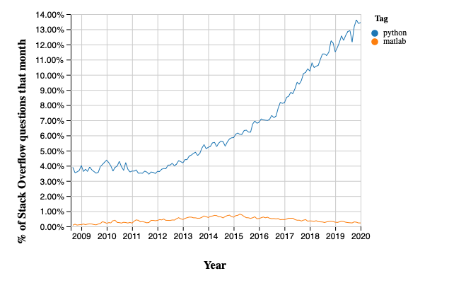
The figure indicates not only that Python is widely used but also that adoption of Python has accelerated significantly since 2012.
We suspect this is driven at least in part by uptake in the scientific domain, particularly in rapidly growing fields like data science.
For example, the popularity of pandas, a library for data analysis with Python has exploded, as seen here.
(The corresponding time path for MATLAB is shown for comparison)
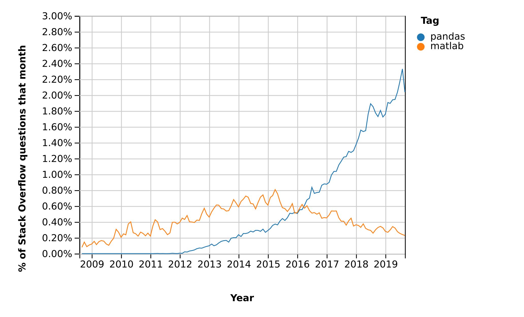
Note that pandas takes off in 2012, which is the same year that we see Python’s popularity begin to spike in the first figure.
Overall, it’s clear that
Python is one of the most popular programming languages worldwide.
Python is a major tool for scientific computing, accounting for a rapidly rising share of scientific work around the globe.
Features
Python is a high-level language suitable for rapid development.
It has a relatively small core language supported by many libraries.
Other features of Python:
multiple programming styles are supported (procedural, object-oriented, functional, etc.)
it is interpreted rather than compiled.
Syntax and Design
One nice feature of Python is its elegant syntax — we’ll see many examples later on.
Elegant code might sound superfluous but in fact it’s highly beneficial because it makes the syntax easy to read and easy to remember.
Remembering how to read from files, sort dictionaries and other such routine tasks means that you don’t need to break your flow in order to hunt down correct syntax.
Closely related to elegant syntax is an elegant design.
Features like iterators, generators, decorators and list comprehensions make Python highly expressive, allowing you to get more done with less code.
Namespaces improve productivity by cutting down on bugs and syntax errors.
Scientific Programming
Python has become one of the core languages of scientific computing.
It’s either the dominant player or a major player in
Its popularity in economics is also beginning to rise.
This section briefly showcases some examples of Python for scientific programming.
All of these topics will be covered in detail later on.
Numerical Programming
Fundamental matrix and array processing capabilities are provided by the excellent NumPy library.
NumPy provides the basic array data type plus some simple processing operations.
For example, let’s build some arrays
import numpy as np                     # Load the library

a = np.linspace(-np.pi, np.pi, 100)    # Create even grid from -π to π
b = np.cos(a)                          # Apply cosine to each element of a
c = np.sin(a)                          # Apply sin to each element of a
Now let’s take the inner product
b @ c
4.04891256782214e-16
The number you see here might vary slightly but it’s essentially zero.
(For older versions of Python and NumPy you need to use the np.dot function)
The SciPy library is built on top of NumPy and provides additional functionality.
For example, let’s calculate \(\int_{-2}^2 \phi(z) dz\) where \(\phi\) is the standard normal density.
from scipy.stats import norm
from scipy.integrate import quad

ϕ = norm()
value, error = quad(ϕ.pdf, -2, 2)  # Integrate using Gaussian quadrature
value
0.9544997361036417
SciPy includes many of the standard routines used in
See them all here.
Graphics
The most popular and comprehensive Python library for creating figures and graphs is Matplotlib, with functionality including
plots, histograms, contour images, 3D graphs, bar charts etc.
output in many formats (PDF, PNG, EPS, etc.)
LaTeX integration
Example 2D plot with embedded LaTeX annotations
Example contour plot

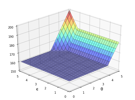
Example 3D plot
More examples can be found in the Matplotlib thumbnail gallery.
Other graphics libraries include
Symbolic Algebra
It’s useful to be able to manipulate symbolic expressions, as in Mathematica or Maple.
The SymPy library provides this functionality from within the Python shell.
from sympy import Symbol

x, y = Symbol('x'), Symbol('y')  # Treat 'x' and 'y' as algebraic symbols
x + x + x + y
We can manipulate expressions
expression = (x + y)**2
expression.expand()
solve polynomials
from sympy import solve

solve(x**2 + x + 2)
[-1/2 - sqrt(7)*I/2, -1/2 + sqrt(7)*I/2]
and calculate limits, derivatives and integrals
from sympy import limit, sin, diff

limit(1 / x, x, 0)
limit(sin(x) / x, x, 0)
diff(sin(x), x)
The beauty of importing this functionality into Python is that we are working within a fully fledged programming language.
We can easily create tables of derivatives, generate LaTeX output, add that output to figures and so on.
Statistics
Python’s data manipulation and statistics libraries have improved rapidly over the last few years.
Pandas
One of the most popular libraries for working with data is pandas.
Pandas is fast, efficient, flexible and well designed.
Here’s a simple example, using some dummy data generated with Numpy’s
excellent random functionality.
import pandas as pd
np.random.seed(1234)

data = np.random.randn(5, 2)  # 5x2 matrix of N(0, 1) random draws
dates = pd.date_range('28/12/2010', periods=5)

df = pd.DataFrame(data, columns=('price', 'weight'), index=dates)
print(df)
               price    weight
2010-12-28  0.471435 -1.190976
2010-12-29  1.432707 -0.312652
2010-12-30 -0.720589  0.887163
2010-12-31  0.859588 -0.636524
2011-01-01  0.015696 -2.242685
df.mean()
price     0.411768
weight   -0.699135
dtype: float64
Other Useful Statistics Libraries
statsmodels — various statistical routines
scikit-learn — machine learning in Python (sponsored by Google, among others)
pyMC — for Bayesian data analysis
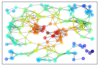
Networks and Graphs
Python has many libraries for studying graphs.
One well-known example is NetworkX. Its features include, among many other things:
standard graph algorithms for analyzing networks
plotting routines
Here’s some example code that generates and plots a random graph, with node color determined by shortest path length from a central node.
import networkx as nx
import matplotlib.pyplot as plt
%matplotlib inline
np.random.seed(1234)

# Generate a random graph
p = dict((i, (np.random.uniform(0, 1), np.random.uniform(0, 1)))
         for i in range(200))
g = nx.random_geometric_graph(200, 0.12, pos=p)
pos = nx.get_node_attributes(g, 'pos')

# Find node nearest the center point (0.5, 0.5)
dists = [(x - 0.5)**2 + (y - 0.5)**2 for x, y in list(pos.values())]
ncenter = np.argmin(dists)

# Plot graph, coloring by path length from central node
p = nx.single_source_shortest_path_length(g, ncenter)
plt.figure()
nx.draw_networkx_edges(g, pos, alpha=0.4)
nx.draw_networkx_nodes(g,
                       pos,
                       nodelist=list(p.keys()),
                       node_size=120, alpha=0.5,
                       node_color=list(p.values()),
                       cmap=plt.cm.jet_r)
plt.show()
Cloud Computing
Running your Python code on massive servers in the cloud is becoming easier and easier.
A nice example is Anaconda Enterprise.
See also
The Google App Engine (Python, Java, PHP or Go)
Parallel Processing
Apart from the cloud computing options listed above, you might like to consider
The Starcluster interface to Amazon’s EC2.
GPU programming through PyCuda, PyOpenCL, Theano or similar.
Other Developments
There are many other interesting developments with scientific programming in Python.
Some representative examples include
Learn More
Browse some Python projects on GitHub.
Read more about Python’s history and rise in popularity.
Have a look at some of the Jupyter notebooks people have shared on various scientific topics.
Visit the Python Package Index.
View some of the questions people are asking about Python on Stackoverflow.
Keep up to date on what’s happening in the Python community with the Python subreddit.